What is a CBEI?
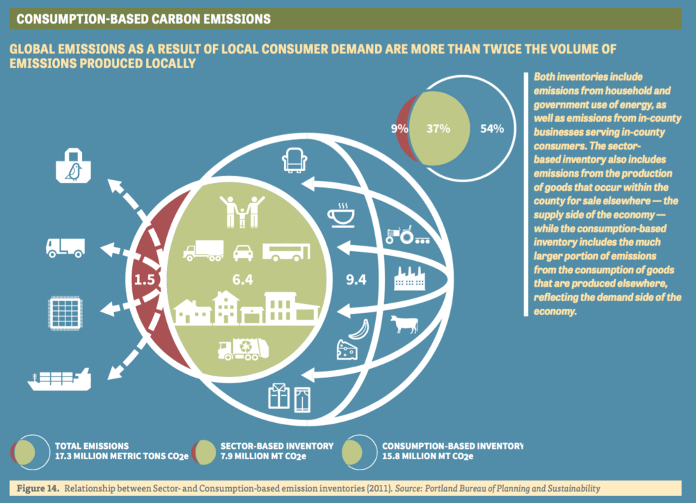
A consumption-based emissions inventory (CBEI) is a calculation of all of the greenhouse gas emissions associated with producing, transporting, using, and disposing of products and services consumed by a particular community or entity in a given time period (typically a year). A CBEI is a way to tally up a comprehensive emissions ‘footprint’ of a community.
A CBEI is not a substitute for a territorial GHG inventory. Rather, the two should be used together
Many local governments already collect data on emissions inside city boundaries. These territorial (or sector-based) inventories are generally best-suited to track emissions, and inform policies, related to energy use in buildings and transportation, along with emissions from in-city industrial and waste sources. A CBEI is most useful for understanding where “embedded” emissions generated outside city boundaries constitute a significant portion of the carbon footprint of household and government consumption. These embedded GHG sources include all the emissions associated with the production, transportation, distribution, and disposal of consumed goods and services. A CBEI can lead to insights about where local consumption gives rise to emissions outside a city’s borders, and suggest additional opportunities for reducing emissions.
Precise calculations of consumption emissions are difficult, but CBEIs provide reasonable estimates
At the most basic level, the calculation of a CBEI entails two main inputs: a measure of what is consumed, multiplied by a measure of how many GHG emissions are associated with each unit of consumption. For example, if a community consumes one million tons of cement each year, and producing and transporting each ton of cement released 1 ton of CO2, the community’s CBEI would include 1 million tons CO2 associated with cement consumption, regardless of whether that cement was produced inside or outside the community’s jurisdictional boundaries. The same basic approach would apply for a unit of any other product or service, whether that be broccoli (also about 1 ton CO2 per ton of broccoli), beef (more like 20 tons CO2 per ton of beef), or ballet tickets.
A full CBEI would, in principle, do something similar for all of the products and services consumed in a city. However, this can prove challenging in practice, because calculating consumption-related emissions precisely is highly complex. Communities consume thousands of different types of products and services, and the emissions associated with each of these is affected by many decisions made by different actors throughout their life cycles. It would take a substantial amount of effort to understand the emissions associated with every consumption decision to create an accurate CBEI—and any precise estimate is likely to become obsolete as production processes and supply chains change over time (sometimes month-to-month or week-to-week).
Fortunately, cities can now produce relatively simple estimates for CBEIs, thanks to recent innovations in the tools available. Furthermore, enough CBEIs have been completed by cities (including in a recent study by C40 Cities) to enable insights about what kinds of policy-relevant information can be distilled even where methods are less precise or have limited resolution with respect to different categories of consumption.
Key CBEI insights
For most cities (at least those cities without substantial heavy industry within their borders) a consumption-based inventory is likely to be substantially higher than a typical, territorial greenhouse gas emissions inventory.
This is because the emissions associated with goods consumed in cities are often released outside the city during production and transportation, e.g., in the course of mining or growing raw materials, processing and manufacturing these materials into products, and packaging and delivering them to consumers. The chart below shows that a CBEI for cities in North America (U.S. and Canada) is likely to be about twice as high as territorial emissions associated with local transportation, buildings, power, industry (if any), and waste. As territorial emissions in many European cities are even smaller (on a per-person basis), the ratio of consumption-based to territorial emissions in European cities can be even larger.
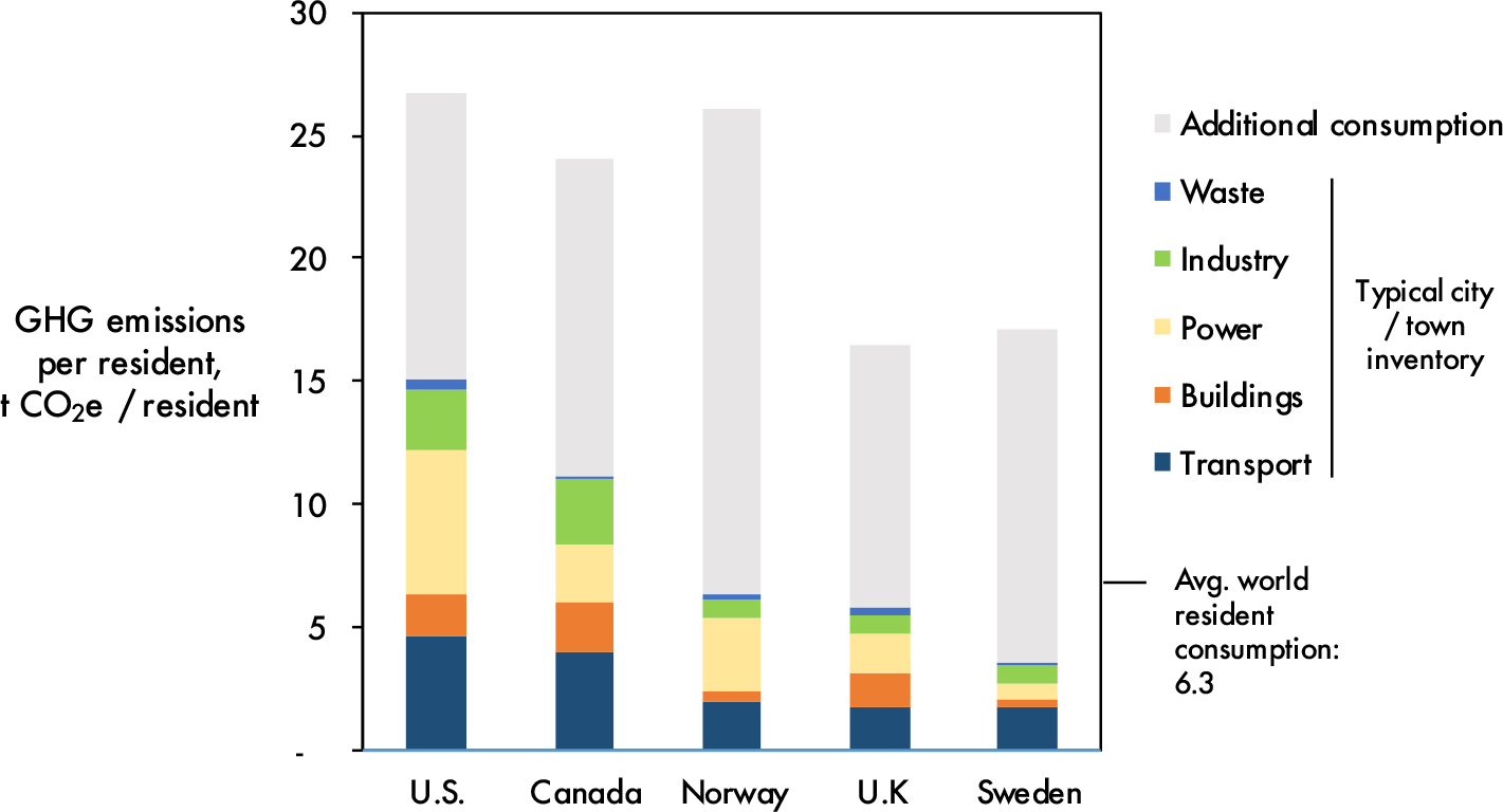
For cities in relatively wealthy, industrialized countries, the full footprint of residents’ consumption is far higher than the global average. The chart above shows that consumption-based emissions associated with residents in the U.S., Canada, Norway, UK, and Sweden are all at least twice as high—and up to four times as high—as the global average. This implies that the responsibility for global GHG emissions and climate change is not distributed equally.
Certain types of consumption are consistently high in most cities CBEIs. The chart below shows that emissions from car travel, building heating, and power consumption each average at least 2 tons CO2e per person in the U.S. But this is already well known from cities’ standard, territorial GHG emissions inventories. The unique contribution of a CBEI perspective is instead the expanded emphasis placed on goods, food, and services, each of which also is generally responsible for another 2 tons or more of CO2e per person. (Depending on how new building and infrastructure construction are categorized, these too could meet this threshold).
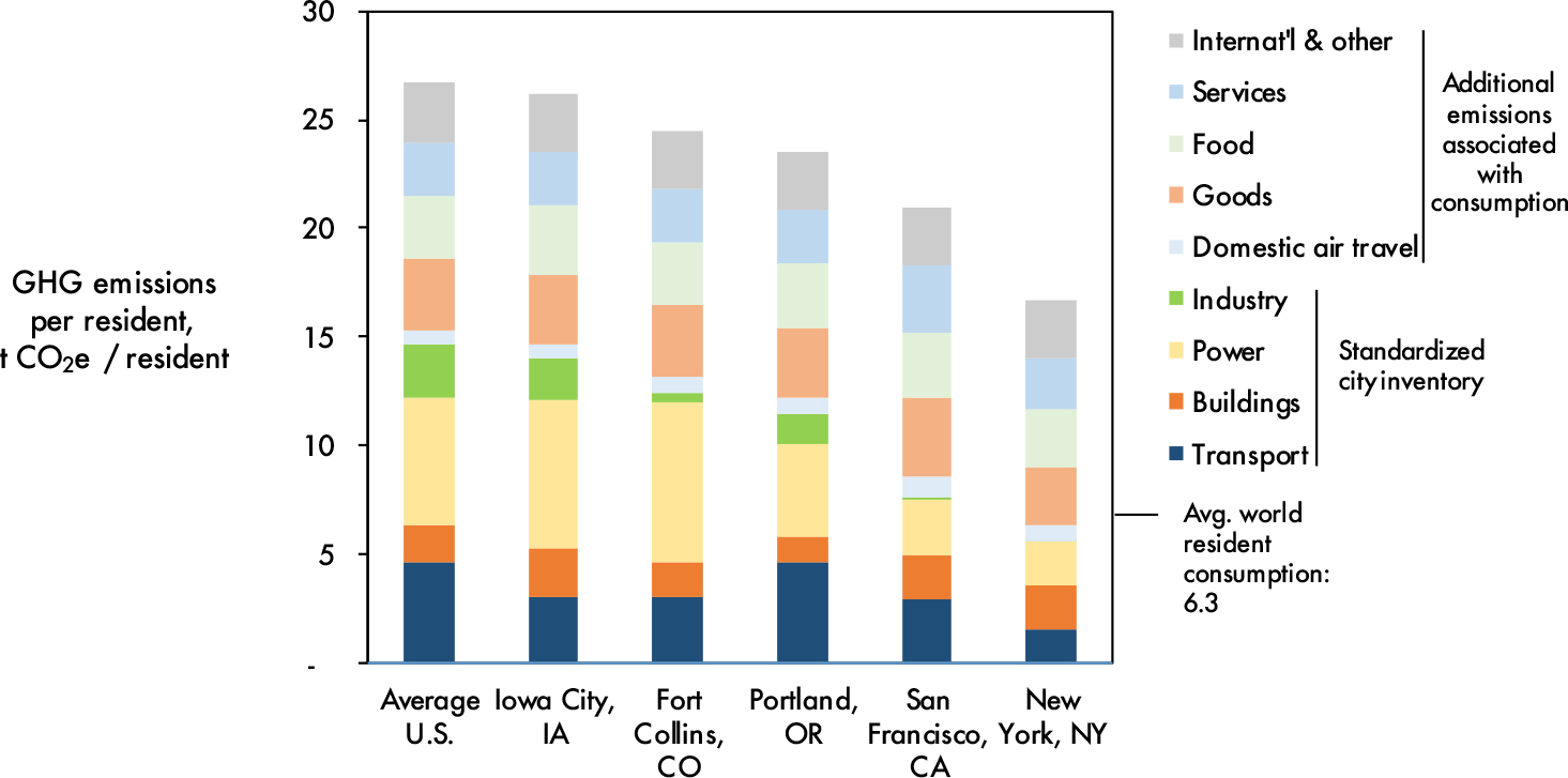
These findings hold true for cities in other high-income countries, as well. For example, a detailed study[3] of subnational regions in the European Union found that consumption-based emissions for food, goods, and services in Berlin, Copenhagen, and London also amounted to at least 2 tons CO2e per person in each of those categories, similar to in the U.S.
CBEIs provide useful insights, but they can paint an incomplete picture of urban emissions patterns. Most CBEIs lump consumption into categories, which can mask the fact that some goods are more emissions intensive than others (e.g. meat production has a larger emissions footprint than other types of food).[4] Such categorization also treats all residents’ consumption as equal, whereas in reality, consumption levels tend to vary widely within cities (e.g. research shows that high-income households typically have a larger consumption footprint than lower-income households).[5] In addition, the majority of emissions associated with different goods and services can occur at different life-cycle phases (e.g. for food, most emissions are associated with production, whereas for appliances the majority of emissions result from use).[6] These distinctions can be important when considering and prioritizing policy interventions.
- Estimates of a typical city/town inventory are based on each country’s national GHG emissions inventory as submitted to the United Nations Framework Convention on Climate Change (UNFCCC), combined with country population data from the World Bank’s Development Indicators. To approximate the emissions associated with a typical city or town GHG emissions inventory, we compiled the emissions from the national inventories that are mostly commonly included in city inventories and that are more strongly associated with urban economies. These included the following emissions inventory ccategories, which are readily reported in national inventories following IPCC accounting protocols:(IPCC 2006) 1A1 (Power), 1A2 (Manufacturing), 1A3b (Road Transport), 1A4 (Buildings), and 5A (Waste). Emissions associated with consumption based on the Eora global multiregional input-output database. Average world resident consumption based on the EDGAR dataset maintained by the European Commission
- Estimates of a typical city/town inventory drawn from U.S. Department of Energy National Renewable Energy Lab (NREL)’s City Energy Profile tool, supplemented with estimates of additional emissions associated with consumption from coolclimate.org, and combined with population estimates from the U.S. Census Bureau’s American Community Survey.
- Ivanova, D., Vita, G., Steen-Olsen, K., Stadler, K., Melo, P. C., Wood, R. and Hertwich, E. G. (2017). Mapping the carbon footprint of EU regions. Environmental Research Letters, 12(5). 054013.
- Ripple, W. J., Smith, P., Haberl, H., Montzka, S. A., McAlpine, C. and Boucher, D. H. (2014). Ruminants, climate change and climate policy. Nature Climate Change, 4(1). 2–5.
- Jones, C. M. and Kammen, D. M. (2011). Quantifying Carbon Footprint Reduction Opportunities for U.S. Households and Communities. Environmental Science & Technology, 45(9). 4088–95.
- Greenhouse Gas Protocol (2011). Product Life Cycle Accounting and Reporting Standard. WRI and WBCSD, Washington , D.C.